Chapter 3: Feed Forward Neural Net
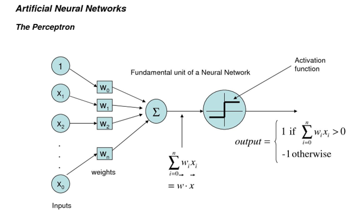
3.1 Perceptron – 신경망
퍼셉트론이란 뉴런을 모방한 회로를 말한다.

다만, 이 퍼셉트론은 선형분류라는 특성상 한계가 존재한다.
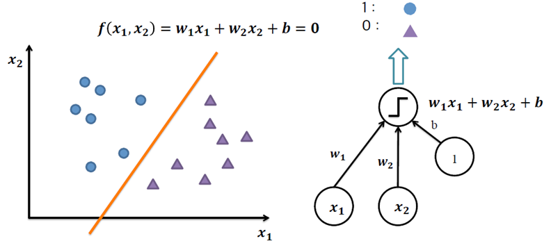
§ 동그라미와 세모를 분리하려면 어떻게 해야 할까?

§ y = ax + b 형태의 직선을 이용할 수 있다.

§ 일반화해서 표현해 보자.

§ Generalization
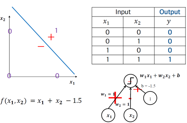
3.1 Perceptron – AND 분류

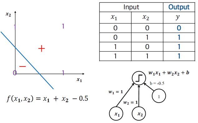
3.1 Perceptron – OR 분류

3.1 Perceptron – XOR 분류
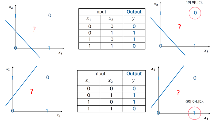
§ Perceptron은 XOR을 분류하지 못한다…
§ 직선 두 개를 이용하여 XOR 분류를 해결 할 수 있다.

§ 그러면, 어떤 모델을 이용하여 직선 두 개를 나타낼 수 있을까?

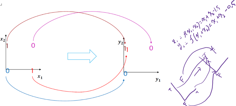
3.2.1 Multi-later Perceptron
§ 여기서 나온 해결책이 MLP로 layer를 추가하면 해결 가능하다.

레이어를 추가하면 아래와 같이 공간이 사상되어 선형 분류가 가능해진다. 다만 이는 svm과의 커널 트릭과는 다름에 유의.

3.2.2 Multi layer Perceptron 학습
§ MLP 학습이란?
• 학습 자료를 이용하여 $W$ 를 추정하는 것이다.

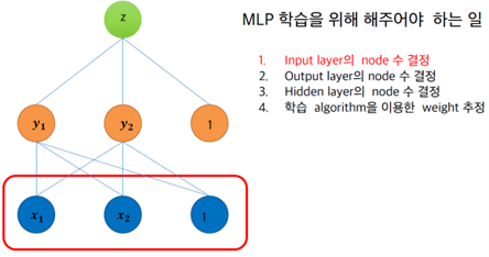
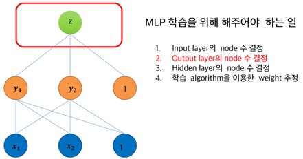
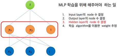
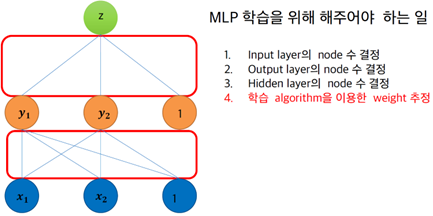
§ MLP 학습을 위해 해주어야 하는 일
• Input layer의 node 수 결정
- Domain에 따라 결정
• Output layer의 node 수 결정
- Domain에 따라 결정한다
• Hidden layer의 node 수 결정
- 실험을 통해 결정
• 학습 algorithm을 이용한 weight 추정
- Back-propagation알고리즘을 이용하여 레이블 된 학습 자료에 최적 weight를 추정한다

3.2.2 Back propagation algorithm
§ 학습은 back propagation 알고리즘으로 수행됨
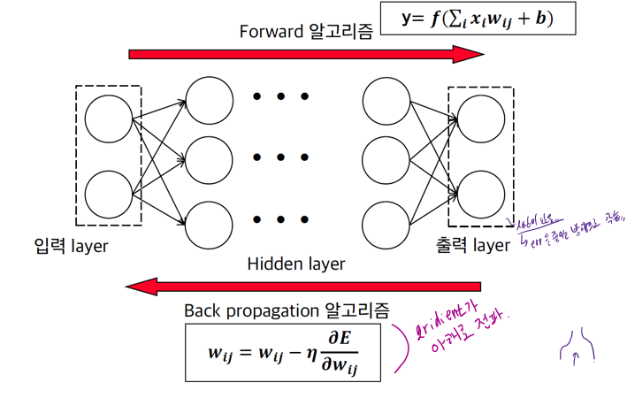
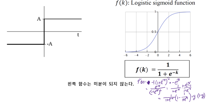
§ Activation 함수로는 sigmoid를 이용한다.
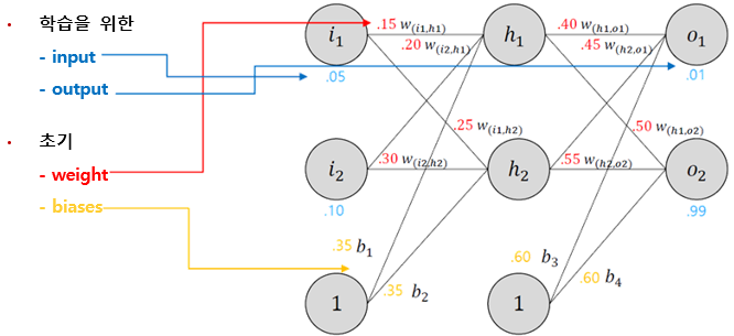
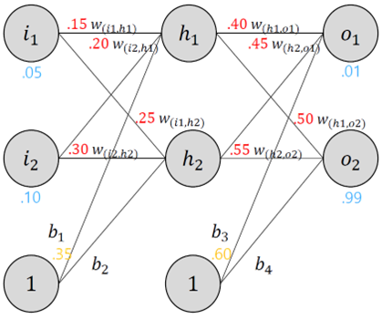
§ 두개의 input, 두개의 hidden neurons, 두개의 output neurons으로 구성된 기본 neural network 구조

§ 예제
§ Backpropagation
• weight들을 최적화하여, 임의의 input/output에 대하여 올바른 답을 낼 수 있도록 함
§ The forward Pass

• $h_{1}$뉴런 input
- $ \text { net }_{h 1}=w_{(i 1, h 1)} * i_1+w_{(i 2, h 1)} * i_2+b_1 * 1 $
- $ \text { net }_{h 1}=0.15 * 0.05+0.3 * 0.1+0.35 * 1=0.38075 $
• logistic function을 거친 $h_{1}$ output
-$\text { out }_{h 1}=\frac{1}{1+e^{- \text {net }_{h 11}}}=\frac{1}{1+e^{-0.3775}}=0.593269992$
• $h_{2}$에 대하여 같은 과정을 반복
-$\text { out }_{h 2}=0.596884378$
• $h_{1}$과 $h_{2}$ 의 방법으로 $o_1$을 진행
-$\text { net }_{o 1}=w_{(h 1,01)} * \text { out }_{h 1}+w_{(h 2,01)} * \text { out }_{h 2}+b 3 * 1$
-$\text { net}_{o 1}=0.4 * 0.593269992+0.45 * 0.596884378+0.6 * 1=1.105905967$
-$\text { out}_{01}=\frac{1}{1+e^{-n e t_{01}}}=\frac{1}{1+e^{-1.105905967}}=0.75136507$
• $o_{1}$의 방법으로 $o_{2}$를 반복
-$\text { out }_{o 2}=0.772928465$
§ Calculating the Total Error
• 앞서 계산된 뉴런의 output을 squared error function의 input으로 에러를 계산
- 수식의 계수 ½ 은 미분의 편의성을 위함. 후 약분 됨.
• 예시
- $o_1$의 target output = 0.01
- $o_1$의 neural net output = 0.75136507
- 따라서, error는 $
\begin{aligned}
E_{o 1} & =\frac{1}{2}\left(\text { target }_{\text {o1 }}-\text { out }_{\text {o1 }}\right)^2 =\frac{1}{2}(0.01-0.75136507)^2 =0.274811083
\end{aligned}
$
§ The Backwards Pass
• Back propagation의 목표인 weight update를 진행
§ Output Layer
• The backwards pass
• 예를 들어, $w_{(h_{1},o_{1})}$를 update 한다면
- total error에 어느정도 영향을 주는지 알기 위해 편미분을 진행 (체인 룰 적용)
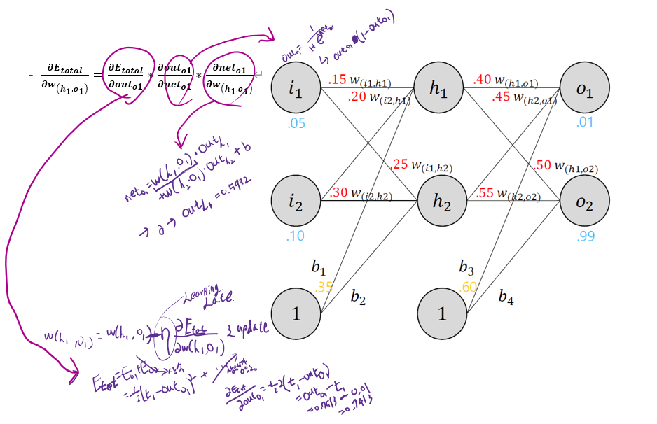
• 위 내용을 시각화 하면 아래와 같다
• 각 부분별로 계산을 진행
• $
\frac{\partial E_{\text {total }}}{\partial w_{\left(h_1, \omega_1\right)}} * \frac{\partial \text { out }_{a 1}}{\partial \text { net }_{o 1}} * \frac{\partial E_{\text {total }}}{\partial o u t_{o 1}}=\frac{\partial E_{\text {total }}}{\partial w_{\left(h_1, \omega_1\right)}}
$

• 먼저, output($o_1$)의 변화에 대한 total error의 변화를 계산
-$
E_{\text {total }}=\frac{1}{2}\left(\text { target }_{01}-\text { out }_{01}\right)^2+\frac{1}{2}\left(\text { target }_{02}-o u t_{02}\right)^2
$
-$
\frac{\partial E_{\text {total }}}{\partial \text { out }}=2 * \frac{1}{2}\left(\text { target }_{o 1}-\text { out }_{01}\right)^{2-1} *-1+0
$
-$
\frac{\partial E_{\text {totai }}}{\text { out }_{01}}=-\left(\text { target }_{01}-\text { out }_{01}\right)=-(0.01-0.75136507)=0.74136507
$
• total net input의 변화에 대한 output($o_1$)의 변화를 계산
- logistic function의 편미분 결과는 $out(1-out)$임
- $
\text { out }{ }_{o 1}=\frac{1}{1+e^{-n e t}}
$
-$
\frac{\partial o u t_{o 1}}{\partial e_{o 1}}=\text { out }_{o 1}\left(1-\text { out }_{o 1}\right)=0.75136507(1-0.75136507)=0.186815602
$
• 그리고, $w_{()}$의 변화에 대한 의 변화를 계산
-$
\text { net }_{o 1}=w_{(h 1, o 1)} * \text { out }_{h 1}+w_{(h 2, o 1)} * \text { out }_{h 2}+b_2 * 1
$
- $
\frac{\partial n e t_{o 1}}{\partial w_{(\hbar 1,01)}}=1 * \text { out }_{h 1} * w_{\left(h_1, o_1\right)}^{(1-1)}+0+0=\text { out }_{h 1}=0.593269992
$
• 위 결과 식들을 종합
- $w_{(h_1,o_1)}$ 의 변화에 대한 total error
*$
\frac{\partial E_{\text {total }}}{\partial w_{\left(h_1, o_1\right)}}=\frac{\partial E_{\text {total }}}{\partial o u t_{o 1}} * \frac{\partial o u t_{o 1}}{\partial \text { net }_{o 1}} * \frac{\partial \text { net }_{o 1}}{\partial w_{(h 1, o 1)}}
$
*$
\frac{\partial E_{\text {total }}}{\partial w_{(\hbar 1,01)}}=0.74136507 * 0.186815602 * 0.593269992=0.082167041
$
• error를 감소시키기 위해, 위 식에서 얻은 값을 현재 weight에서 빼준다. 이때 learning rate(eta)을 곱한 뒤 뺀다.
-$
w_{\left(h_1, 0_1\right)}^{+}=w_{\left(h_1, 0_1\right)}-\eta * \frac{\partial E_{\text {total }}}{\partial w_{\left(h_1, 0_1\right)}}=0.4-0.5 * 0.082167041=0.35891648
$
• 동일한 프로세스를 $w^{+}_{(h_1, o_1)}~w^{+}_{(h_2,o_2)}$에 대하여 반복
-$
w_{\left(h_2, o_1\right)}^{+}=0.408666186
$
-$
w_{\left(h_1, o_2\right)}^{+}=0.511301270
$
-$
w_{\left(h_2, 0_2\right)}^{+}=0.561370121
$
• weight값 실제 update는 hidden layer에 대해서 새로운 weight을 모두 구한 후 update를 진행

§ Hidden Layer
• The backwards pass (Cont.)
- $w_{(i_1, h_1)}~w_{(i_2, h_2)}$에 대해서 값을 계산
• output layer에서 진행했던 방식과 유사한 방식
- 차이점 : 여러 개의 output neurons의 변화량 사용
⁎ $h_1$의 out부분이 $o_1, o_2$에 영향을 줌
$
\frac{\partial E_{\text {total }}}{w_{(i 1, \boldsymbol{h} \mathbf{1})}}=\frac{\partial E_{\text {total }}}{\partial o u t_{h \mathbf{1}}} * \frac{\partial o u t_{\boldsymbol{h} \mathbf{1}}}{\partial n e t_{\boldsymbol{h} 1}} * \frac{\partial \text { net }_{\boldsymbol{h} \mathbf{1}}}{\partial w_{(i 1, \boldsymbol{h} \mathbf{)}}}
$
**$
\frac{\partial E_{\text {total }}}{\partial o u t_{h 1}}=\frac{\partial E_{o 1}}{\partial o u t_{h 1}}+\frac{\partial E_{o 2}}{\partial o u t_{h 1}}
$

§ Hidden Layer (Cont.)
• $
\frac{\partial E_{o 1}}{\partial o u t_{h 1}}
$계산시 앞서 계산한 $
\frac{\partial E_{o 1}}{\partial n e t_{h 1}}
$을 사용
-$
\frac{\partial E_{o 1}}{\partial o u t_{h 1}}=\frac{\partial E_{o 1}}{\partial \text { net }_{o 1}} * \frac{\text { net }_{o 1}}{\partial o u t_{h 1}}
$
-$
\frac{\partial E_{01}}{\partial n e t_{o 1}}=\frac{\partial E_{01}}{\partial o u t_{o 1}} * \frac{\partial o u t_{o 1}}{\partial n e t_{01}}=0.74136507 * 0.186815602=0.138498562
$
• $
\frac{\partial n e t_{o 1}}{\partial o u t_{h 1}}
$와 $w_{(h_1, o_1)}$이 같으므로
-$
\text { net }_{o 1}=w_{(h 1, o 1)} * \text { out }_{h 1}+w_{(h 2,01)} * \text { out }_{h 2}+b 3 * 1
$
-$
\frac{\partial n e t_{o 1}}{\partial o u t_{h 1}}=w_{(h 1, o 1)}=0.40
$
• 위 식들을 합쳐주면
-$
\frac{\partial E_{o 1}}{\partial \text { out }_{h 1}}=\frac{\partial E_{o 1}}{\partial \text { net }_{o 1}} * \frac{\partial n e t_{o 1}}{\partial \text { out }_{h 1}}=0.138498562 * 0.40=0.055399425
$
• 같은 방식으로 $
\frac{\partial E_{o 2}}{\partial o u t_{h 1}}
$를 계산
⁻$$
\frac{\partial E_{o 2}}{\partial \text { out }}=-0.019049119
$$
• 따라서 $
\frac{\partial E_{\text {total }}}{\partial o u t_{h 1}}
$계산 가능
⁻$
\frac{\partial E_{\text {total }}}{\partial \text { out }_{h 1}}=\frac{\partial E_{o 1}}{\partial o u t_{h 1}}+\frac{\partial E_{o 2}}{\partial o u t_{h 1}}=0.055399425+-0.019049119=0.036350306
$
• $
\frac{\partial E_{\text {total }}}{\partial o u t_{h 1}}
$를 얻었으므로, 각 weight에 대해 $
\frac{\text { oout }_{h 1}}{\partial \text { net }_{h 1}}
$와 $
\frac{\partial n e t_{h 1}}{\partial w}
$를 계산
-$
\text { out }_{\boldsymbol{h} \mathbf{1}}=\frac{1}{1+e^{- \text {net }_{h 1}}}
$$
-$
\frac{\text { ouut }_{h 1}}{\partial \text { net }_{h 1}}=\text { out }_{h 1}\left(1-\text { out }_{h 1}\right)=0.59326999(1-0.59326999)=0.241300709
$
• output 뉴런에서 했던 방식을 적용하여, $w_{(i_1, h_1)}$에 대한 total net input to $h_1$ 의 편미분을 계산
-$
\text { net }_{h 1}=w_{(i 1, h 1)} * i_1+w_{(i 2, h 1)} * i_2+b 1 * 1
$
-$
\frac{\partial n e t_{h 1}}{\partial w_{(i 1, h 1)}}=i_1=0.05
$
• 위 식을 모두 합치면$
\frac{\partial E_{\text {total }}}{\partial w_{(i 1, h 1)}}=\frac{\partial E_{\text {total }}}{\partial o u t_{h 1}} * \frac{\partial o u t_{h 1}}{\partial n e t_{h 1}} * \frac{\partial n e t_{h 1}}{\partial w_{(i 1, h 1)}}
$
-$
\frac{\partial E_{\text {total }}}{\partial w_{\left(i_1, h_1\right)}}=0.036350306 * 0.241300709 * 0.05=0.000438568
$
• $w_{(i_1, h_1)}$을 update
-$
w_{\left(i_1, h_1\right)}^{+}=w_{\left(w_1, h_1\right)}-\eta \frac{\partial E_{\text {total }}}{\partial w_{\left(i_1, h_1\right)}}=0.15-0.5 * 0.000438568=0.149780716
$
• 같은 방법으로 $
w_{\left(i_2, h_1\right)}^{+} \sim w_{\left(i_2, h_2\right)}^{+}
$ 를 반복
-$
w_{\left(i_2, h_1\right)}^{+}=0.19956143
$
-$
w_{\left(i_1, h_2\right)}^{+}=0.24975114
$
-$
w_{\left(i_2, h_2\right)}^{+}=0.29950229
$
§ 학습 결과 예제
• 1st error = 0.298371109
• 2nd error = 0.291027924
- …
- …
• 10000th error = 0.00035085
- 이때, 두 output 뉴런을 보면,
* 0.015912196 (vs 0.01 target)
* 0.984065734 (vs 0.99 target)
'IT > 수업내용 정리' 카테고리의 다른 글
| ASR_Chpter 05: Sequence-to-Sequence with Attention (0) | 2024.10.28 |
|---|---|
| ASR_Chapter 4: Recurrent Neural Networks (0) | 2024.08.14 |
| pattern recognition_Ch 02 Bayesian Decision Theory (1) | 2022.12.21 |
| pattern recognition_ch01 Intro (0) | 2022.12.21 |
| ASR_Chapter 2: 입/출력 end 복잡도 분석 (3) | 2022.11.18 |